
Menu
EWOC Web Portal EWOC Web Portal Sign Up
documentation
(PDF)
(PDF)
(MS Word) (MS Word Doc)
(EndNote)
download
contact us
Link EWOC CRAN Packages
release notes

User Guide
Contents
I. Description of the Integrated Web Portal
II. Getting Started
III. Running EWOC - Dose Computation
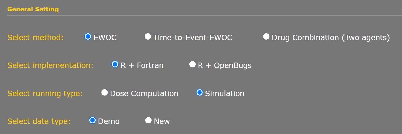
1. General Settings
Select Method
Select Implementation
Select Running Type
Select Data Type
2. Required parameters
Probability of dose limiting toxicity (θ)
Probability of exceeding the Target dose (α)
Minimum dose
Maximum dose
Matrix Input
3. Optional fields
Title
Minimum dose increment
Bayesian confidence interval
Marginal posterior distribution plot
Cohort size
Tree of doses for next Cohort
Variable Alpha Increment
Sequence of Doses with no DLTs
4. Prior Distributions
For the Probability of DLT at Initial Dose ρ0
For the Maximum Tolerated Dose (γ) dose
5. Extended Prior Distributions
6. Results
Exporting output
IV. Running Time-to-Event-EWOC Dose Computation
1. Required parameters
DLT Assessment Window
Matrix Input
2. Optional Fields
3. Prior Distributions
4. Extended Prior Distributions
5. Results
V. Running Drug Combinations (Two Agents)
1. General Settings for Drug Combination Methods
4. Required Parameters
2. Optional Fields
3. Prior Distributions
5. Results
VI. Example Output - Dose Computations
1. Example 1 - Discrete Doses
Bayesian confidence interval
Marginal posterior distribution plot
Tree of doses
2. Example 2 - Continuous dosing schema
3. Example 3 - Time-to-Event Dose Computation
4. Example 4 - Two Drug Combination Studies
VII. Running EWOC - Trial Simulation Mode
1. Simulation Setup
2. Scenario Setup for Continuous Doses
3. Scenario Setup for Discrete Doses - Specifying the Level of MTD
4. Scenario Setup for Discrete Doses - Probability of DLT at Dose Levels
5. Simulation Setup - Priors & Extended Priors Tabs
6. Running Simulation - Results
VIII. Running Time-to-Event-EWOC – Trial Simulation Mode
1. Simulation Setup
2. Running Time-to-Event Simulation - Results
IX. Appendix
1. EWOC Mathematical Formulation
2. WEB-EWOC High Level Systems Architecture
3. Database Scheme
X. References
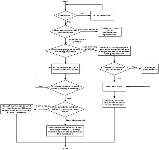
I. Description of the Integrated Web Portal
The integrated Web portal for Escalation with Overdose Control (EWOC) is an industry-standards based, database-driven, distributed computing platform for designing and conducting dose finding in clinical trials in cancer using the EWOC method.
The integrated Web portal provides two ways to the registered users to utilize the software:
- Web-based calculators which is database-driven, client/server, multiuser-based architecture. It is developed using open source software and running on the Linux-Apache Web server. The Web interface is implemented using PHP, JavaScript and jQuery for full user-input validation; the middleware is also developed in PHP to connect Web interface and backend R+OpenBugs and R+Fortran code which realizes core EWOC algorithm and Oracle database.
- Standalone downloadable application which is implemented in Fortran programming language and currently it can run on the Windows operating system.
The integrated Web portal for EWOC provides secure, database-driven, user-friendly interface for EWOC method. The Web-based interface calculator not only provides the way to calculate next dose but also provide the way to calculate Beta prior distribution. The calculating results are also stored to the backend database which is only retrievable by the user who created the project and task. Next time when this user logs into the system, he/she can choose to start the new project or continue with the stored previous running project.
Please see the Appendix for further details regarding the system architecture and database schema.
Web-EWOC 1.8 is a web-based application compatible with Internet Explorer 8 and above, Firefox, Chrome, and Safari. It is available at:
- To get started for the first time, you will need to register. Click on
 to register. You will be asked to create a User Name and Password.
 - Enter in your contact information, solve the security code image, read and agree to the "User Disclaimer". The
 box will appear below. Click on it to continue. An auto confirmation email will be sent to you. Once you have successfully created a login, you can enter the site directly from the homepage.
If you forget your User Name or Password, follow the ![]() link to get a reminder email.
link to get a reminder email.
- After 20 minutes of inactivity, the system will auto-logout.
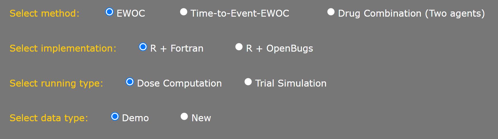
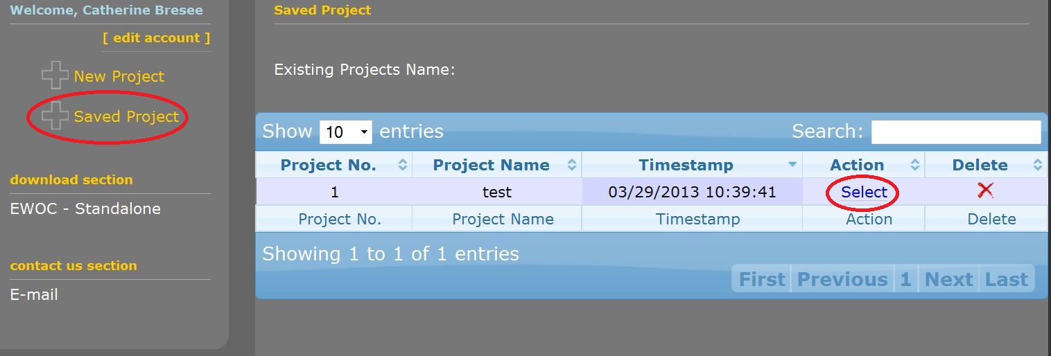
Once you successfully log in, you will be given the choice to either start a new project or open a saved project via the links on the left window:
Your work is saved as Projects and Tasks within each project.
Choose "New Project" to get started for the first time. Enter in a Project Name and Task name and choose "Submit".
- You are able to access and delete your existing projects and tasks via the "Saved Projects" dashboard. To resume work on a saved project, click on "Select" under "Action" on the dashboard.
III. Running EWOC - Dose Computation
- The EWOC-DIALOG will appear after you start a New Project or resume a Saved Project.
To reset your selections back to default values at any time, hit the "F5" key to reload the website page.
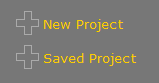
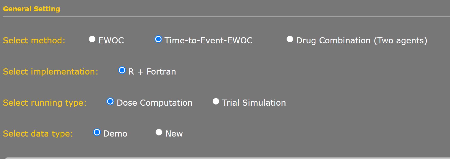
Select Method
Choose "EWOC" option to begin. Please see Section VI for detailed instruction for Time-to-Event-EWOC. or Section VII for Drug Combination
Select Implementation
There are two choices available:
- "R+Fortran" implementation uses numerical integration in computing results, which should be identical to results from the downloadable version of the EWOC program.
- "R+Open Bugs" implementation (original to Web EWOC v1.0) remains an option for users who wish to use Markov Chain Monte Carlo sampling techniques for computations.
Select Running Type
There are two choices available:
- "Dose Computation" will calculate the dose for a single patient or a series of consecutive patients based on previous data and design parameters.
- "Trial Simulation" will simulate a complete trial outcome and generate design operating characteristics for either a continuous dose or a discrete set of increasing doses for a given scenario. (See Section VII for more details.)
Select Data Type
Choosing "Demo" allows preset values to be entered as an example. "New" will allow you to work with a blank interface. "Previous Saved" is chosen when loading parameters from a saved set.
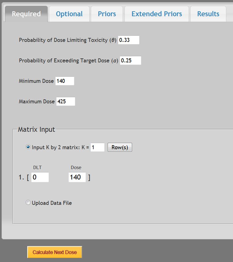
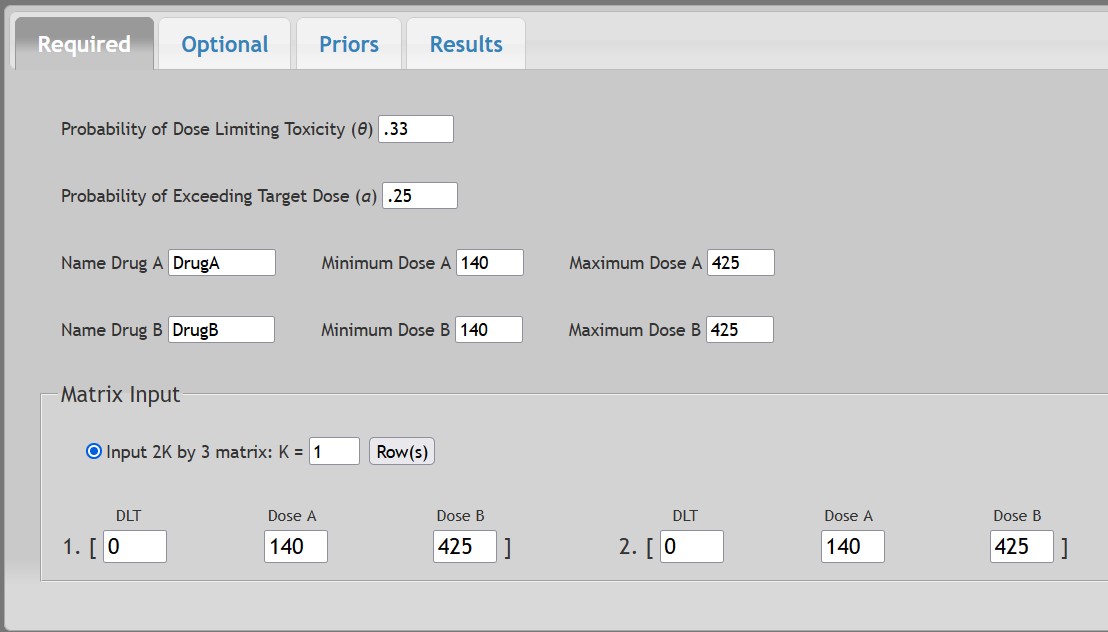
Probability of dose limiting toxicity (θ)
This is the proportion of patients expected to experience a medically unacceptable, dose-limiting toxicity (DLT) if the Target dose (or maximum tolerated dose, MTD) is administered. Its value, generally between 0.1 and 0.5, depends on the nature of the DLT. It would be set relatively high when the DLT is a transient, correctable or non-fatal condition, and low when it is lethal or life threatening. In the dialog window above, the default value is θ = 0.33. NOTE that if the study is designed with an increasing alpha over sequential patients, the value input here will need to reflect the current alpha value, not the initial alpha value at the start of a study.
Probability of exceeding the Target dose (α)
This is the probability that the dose selected by EWOC is higher than the Target dose. Low values make the escalation cautious, high values cause larger steps. In the beginning of a trial, there is a higher level of uncertainty about the Target dose. Consequently, at the onset of a phase I trial, the probability of exceeding the Target dose is typically set to a low value (e.g., 0.25) in order to minimize the possibility of harming patients by administering doses much greater than the Target dose. In the dialog window above, the default value is α = 0.25. As the trial progresses, uncertainty about the Target dose declines and the likelihood of administering a dose considerably higher than the Target dose decreases. Thus, one should consider gradually increasing α during the course of the trial. When the probability of exceeding the Target dose is set to the maximum value of 0.50, it implies that under dosing a patient (treating with a dose lower than the Target dose) is just as bad as overdosing.
Minimum dose
This is the lower bound Xmin of the support of the MTD γ. The dose to be given to the first patient in the trial is always greater than or equal to Xmin. Note that the dose given to the first cohort of patients is not necessarily equal to Xmin but there must be strong evidence that it is a safe dose. EWOC will never assign doses below Xmin. In the dialog window above, the default value is Xmin = 140.
- The Minimum Dose is assumed to be the lowest dose that is known safe without any expected DLT. Should a DLT be observed at this minimum dose, the study should be halted.
Maximum dose
This is the upper bound Xmax of the support of the MTD γ. The highest allowable dose in the trial must be less than or equal to Xmax. EWOC will never assign doses above Xmax. In the dialog window above, the default value is Xmax = 425.
Matrix Input
There are two ways to input your prior patient data.
- The first patient is assumed to receive the Minimum Dose with No DLT.
- A minimum of 1 and a maximum of 100 patient observations can be entered.
A) Input Manually:
![]()
- Each entry of the matrix corresponds to one patient. To add more patient data to the matrix, increase the K = value
- Two values must be entered for each patient data set:
- The first number is either
- The second number is the dose given to this patient. It must be a value between Xmin and Xmax
B) Upload Data file:
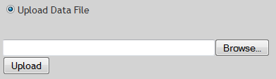
Before running EWOC, a data file (saved in .txt format) containing at least one line must be created. To create a data file, any text editor (e.g., NOTEPAD) can be used. Files also can be created in Microsoft Word and saved with a .txt format.
The data file has the following structure:
- Each line corresponds to one patient.
- Each line must begin with two numbers separated by spaces.
- The first number is either
- The second number is the dose given to this patient.
For example:
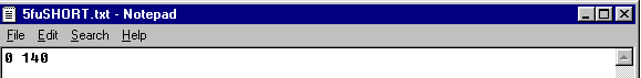
and the following data line:
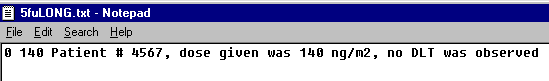
are both valid and equivalent, as interpreted by EWOC.
Note: The text file is considered space delimited. If you accidentally have extra spaces before the first or second value on each line, the data will be considered missing. Also be careful not to mix space delimitation with tab delimitation. Once the file is correctly read in, the Matrix Input fields will be auto-populated for review prior to computation. If the .txt file was not properly configured the upload will be shifted.
3. Optional Fields
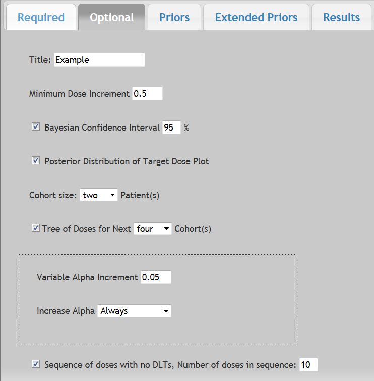
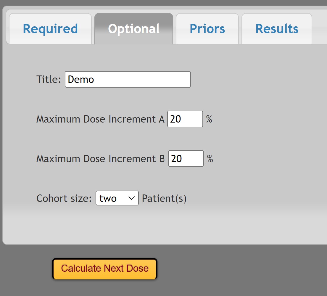
Title
Up to 100 characters can be used to label all output and printable reports, including the Marginal Posterior Distribution Plot and the Tree of Doses.
Minimum Dose increment
Controls how the doses are rounded or truncated. Changes in dose level will be in integer multiples of the selected minimum increment. For example, when the Initial dose is 140 units, a Minimum dose increment of 25 units could possibly produce the sequence of doses: 140, 215, 265, 290 ... From a theoretical perspective, dose varies continuously from Xmin to Xmax. In practice, due to dilution or measurement limitations, it may be possible to obtain only discrete dose levels. When left equal to zero, the next dose will be rounded to three decimal places. Computed dosages are rounded down to the next lowest dose increment.
Bayesian confidence interval
The interval which most likely contains the true Target dose. For example, if [223.2, 425.0] is a Bayesian confidence interval at the 95% level, then the probability that the Target dose lays between 223.2 and 425.0, given the available data, is 0.95. The length of the interval measures the uncertainty about the Target dose. The most frequently used level is 95.0% which is the most common value chosen. EWOC can calculate levels between 4 and 98%.
Marginal posterior distribution plot
Conveys the accumulated information about the Target dose. A Bayesian confidence interval is depicted only when the previous box was also checked.
Cohort size
This option allows you to design a trial with cohorts of p patients at each dose level, p =1, 2, 3. The default is one patient. To select either two or three patients, click the right corner for the drop-down box, and then select either two or three to make the selection, which will then be highlighted. In the example, we selected cohorts of size p = 2.
Tree of doses for next Cohort
This option requests the results display the recommended doses for the next two, three, and four cohorts of p patients depending on the number of DLTs observed for that cohort. The default is to display results for just the next patient. To have the results display the next two to four cohorts, select either three or four cohorts, click the right corner for the drop-down box, and then select two to four to make the selection, which will then be highlighted. In the example, we selected Tree of Doses for next four cohorts of two patients per cohort. Selecting a higher value will decrease computational speed.
Variable Alpha Increment
When running simulations, the probability of exceeding target dose (α) can be gradually increased during the course of the trial to meet the need of a relatively higher probability of exceeding target dose as the trial progresses and the uncertainty about the target dose declines. The cumulative value for alpha will stop once α = 0.5 (the maximum allowable value) (the maximum allowable value). You may also choose to increase the alpha value "Always" or "Only If No DLT" from the drop down menu. When Variable Alpha Increment input value is set to 0 the "Increase Alpha" drop down will default to the "Always" selection, indicating the alpha value will remain constant during the course of the trial.
Sequence of Doses with no DLTs
When this option is selected, the results window will display the dosing sequence for each patient assuming no DLTs are experienced in the study. This is sometimes a useful option to see how large each step in the dosing sequence will be. Note that the dosing sequence can be modulated by adjusting the α (which is the overdose control level).
4. Prior Distributions
We do not recommend changing the defaults for the prior distributions unless you know what you are doing.
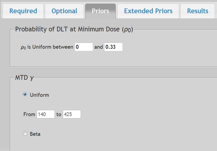
For the Probability of DLT at Initial Dose ρ0
- The default is the uniform distribution between zero and θ, the probability of dose limiting toxicity at the Target dose. The upper limit field changes automatically as θ does. To make them different from each other, change the upper limit field AFTER each change made in θ.
For the Maximum Tolerated Dose (γ) dose
- The default for the MTD is the uniform distribution between Xmin and Xmax
- Alternatively, a Beta distribution can be selected. The prior distribution of the MTD may be specified via one of the three option tabs available:
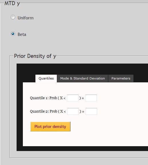
- Quantiles: Based on either prior data or expert opinion, the beta distribution can be estimated from the cumulative distribution function of the MTD at two pre-specified doses (Quantile 1 and Quantile 2). The distribution is estimated by numerical approximation.
- Mode and Standard Deviation: The prior beta distribution of the MTD can be estimated also from a specified mode and SD values for the MTD, if known. The distribution is estimated by numerical approximation.
- Beta Standard Parameters: The distribution can also be estimated by the theoretical parameters values for alpha and beta. The distribution is computed directly from these given parameters.
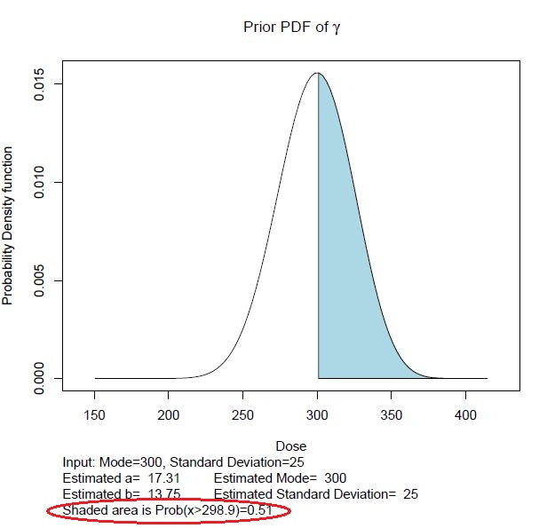
- Select the
 button to accept the values entered to generate the Prior PDF of γ. The
  button is will become available after the prior density is plotted when using the Beta option.
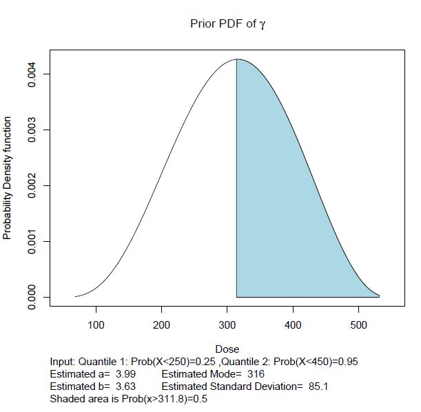
 - After the Prior PDF of γ is generated, the resulting plot is generated. In this example the following parameters were used:
- The probability of x > mode is calculated automatically, and is shaded. To update the quantile value of the estimated probability, enter the desired value to be estimated and select the "Refresh Quantiles" button.
5. Extended Prior Distributions
Additional priors are available for more advanced modeling using distributions as described in Tighiouart et al (2005). Here the major difference is the option to identify the probability of DLT at the minimum dose (ρ0) and the MTD (γ) are either dependent or independent in joint modeling, with the MTD (γ) unbounded from above.
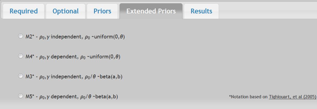
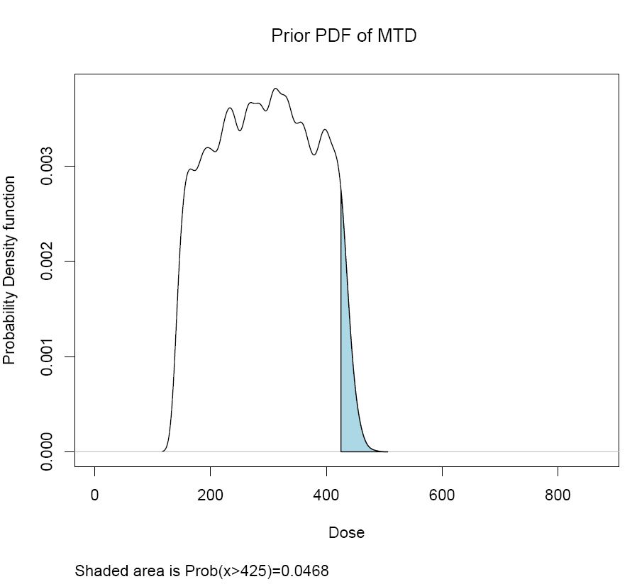
Selection any one of these options will ignore options selected under the other "Priors" tab. You will be prompted to input values for σ1, σ2, and a value for A. where A is the lower bound of the estimated MTD. σ2 controls the degree of flatness of the prior density of the MTD in the interval (Xmin, A) and s1 controls the spread of this density in the interval (A, ∞). A is the quantile of this density corresponding to the prior probability that the MTD exceeds it.
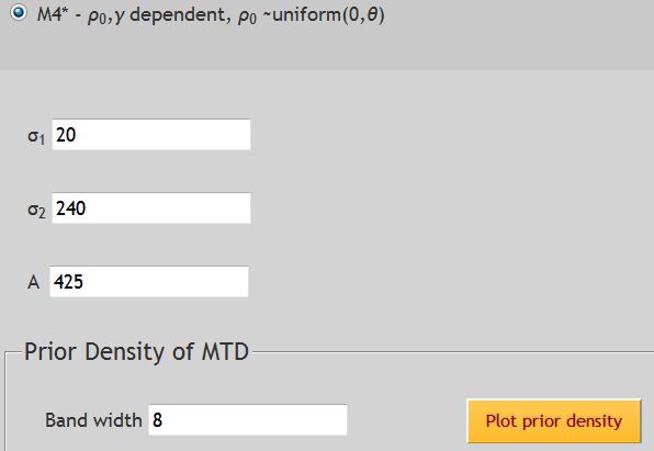
The prior density plot can be smoothed by selecting a higher bandwith.
Given that the MTD is unbounded, the probability of exceeding the value A will be shaded in the plot of the prior density.
See Tighiouart et al, 2005 for a more detailed discussion of all options available under the Extended Priors tab.
Once all parameters are set, choosing ![]() will initiate computation.
will initiate computation.
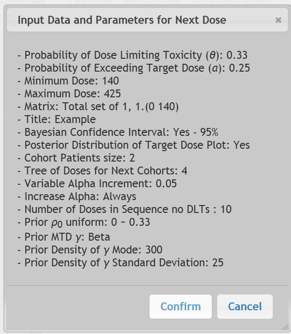
- Any out-of range values will be flagged with an error message prior to continuing computation.
- A confirmation pop-up window will allow final review of all input parameters at which point you may select "Confirm" or "Cancel".
Newly computed results will appear immediately once the "Calculate Next Dose" button is chosen. Up to 3 PDF windows will open with results:
- Report Results: This output window will be displayed for all results. It will include a section of Input Parameters and another section of Results which will include doses for the next patient. If a Sequence of No DLTs is requested, it will appear here.
- Tree of Doses: This output window will be displayed when this option is selected. It will also include a summary of the input parameters.
- Marginal Posterior Probability Density Function: This plot is the marginal posterior probability density function of γ (the MTD) and will change based on the data input under the "Priors" tab.
All results generated for a given project will be automatically saved and can be reviewed under the Results tab. For first time users, this tab will contain no data.
In the following example, both the "Next Dose" results and the prior "Density Plot" files have been saved from one run, as well as the corresponding "Parameters File". All underlined file names can be clicked on to view in a new window.
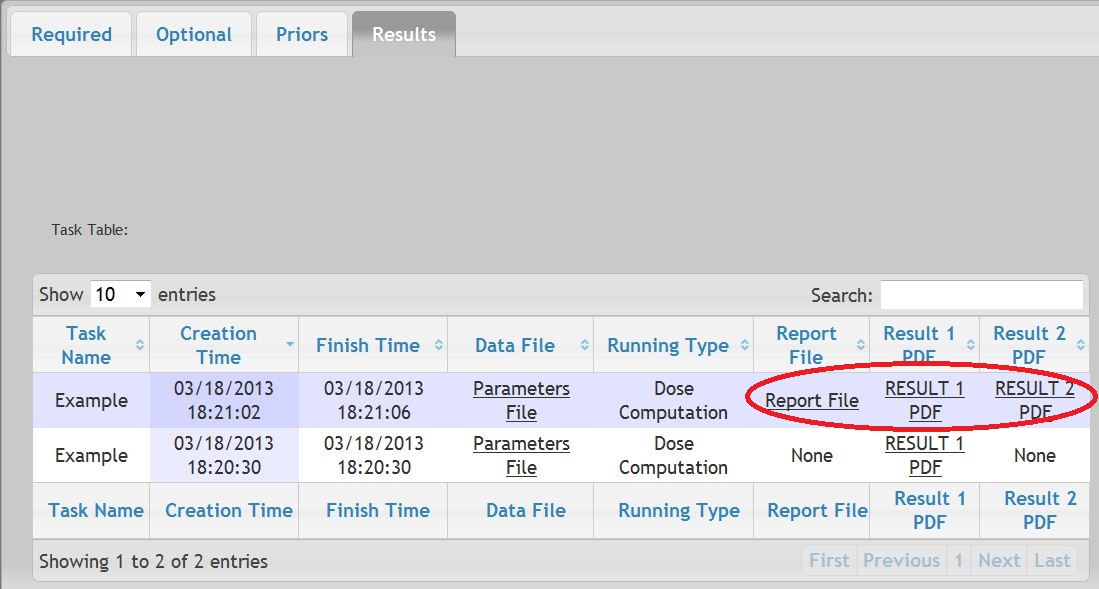
The "Report File" contains the recommended dose for the next scheduled patient along with all parameters. The Tree of Dosing results can be reviewed by selecting "RESULT1" pdf files. The Posterior Distribution of Target Dose Plot is viewable under the "RESULT2" pdf file if such option had been requested.
The parameters chosen for each set of results can be reviewed by selecting the "Parameters File" link.
In the above example, the prior density plot of the MTD was created first and was saved as a separated result file titled "RESULT1".
The Marginal distribution plot and Tree of doses are generated as pdf files. To print or make them available to other applications, click on the window containing the desired output, then click on the Save icon in the pdf file menu. (Note specific icons will vary depending on your browser and Adobe Reader software.)
IV. Running Time-to-Event-EWOC Dose Computation
One limitation of EWOC is that the toxicity outcome is coded as binary as the presence or absence of DLT. However, in some dose finding studies, the observation time to resolve a subject's outcome may be very long. Under the original EWOC design rather than delaying enrolment of a new subject while waiting for the previous subject's results, a new subject would simply be assigned the same dose until additional data could be collected. This limitation motivated the development of models to estimate the MTD that take into account the time subjects are under observation.
Of note, this modeling assumes that should the DLT status of the previously enrolled subject is not known when a new subject is ready to start, then the longer the time the previous subject goes without experiencing a DLT, the higher the recommended dosage would be for the new subject. Correspondingly, should a previous subject experience a DLT shortly after drug administration, then the next dose computed would be lower than if the previous DLT had happened later. We assume the risk of DLT for any given dose follows a Cox proportional hazards model.
(See Tighiouart et al, 2014, for more detailed explanation.)
General Settings - Select Data Type
Choosing "Demo" allows preset values to be entered as an example. "New" will allow you to work with a blank interface. "Previous Saved" is an option that can be chosen when loading parameters from a saved set.
The Required Parameters are similar as described in Section V.2, with the following changes to allow for the observation time to resolve a DLT.
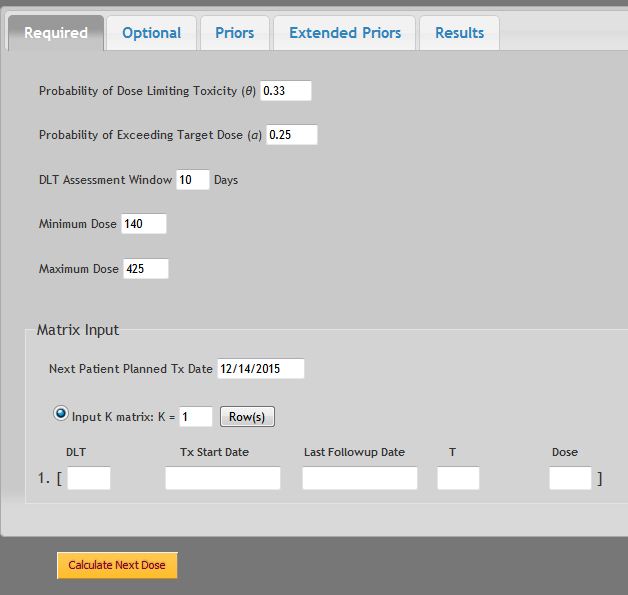
This is the number of days the study protocol allows for a DLT to be resolved. The observation window is defined as (0,τ].
- Input the calendar date the next patient is scheduled to receive the next dose.
- Each entry of the matrix corresponds to one patient. To add more patient data to the matrix, increase the K = value
- The following data must be entered for each patient data set:
- The first number is either
- Enter the calendar date this patient received the recommended dose
- If a DLT was observed during the observation timeframe, enter in the date it occurred. If no DLT was observed, the Last Follow Up Date will be automatically entered as the current date. The total number of days observed (T) will be automatically computed and cannot exceed the number of days assigned for the previously specified "DLT Assessment Window".
- Enter dose given to this patient. It must be a value between Xmin to Xmax.
The Optional Fields that are available are described in Section V.3
Note that in Time-to-Event EWOC, it is always assumed the cohort size will be one. In practice, it would be unrealistic to assume any trial would have >1 subject begins at identical times. As each new patient enrolls, it is assumed some follow-up data would be available on the previous subject and could be used in computing the next dose.
See Section V.4
4. Extended Prior Distributions
See Section V.5
After all data has been input under each tab, selecting the ![]() button will generate two PDF files.
button will generate two PDF files.
1) Report Results: This output window will be displayed for all results. It will include a section of Input Parameters and another section of Results which will include doses for the next patient.
2) Marginal Posterior Probability Density Function: This plot is the marginal posterior probability density function of g (the MTD) and will change based on the data input under the "Priors" tab.
All results generated for a given project will be automatically saved and can be reviewed under the Results tab. For first time users, this tab will contain no data.
V. Running Drug Combinations (Two Agents)
Phase I dose finding trials of two-drug combination therapy traditionally are designed to estimate the MTD of a single drug for a given fixed dosage of the other agent. While results may provide a final safe dose for the combination, the therapeutic effect may be sub-optimal. EWOC can be used for estimating the MTD of two drugs in combination.
In this module EWOC assumes:
- Each drug combination is tested in a cohort of 2 subjects.
- The first cohort of 2 subjects receive the same drug combination dosages of the two drugs at or above the minimum dose of each drug as decided by the study protocol.
- That DLT data are available on each prior cohort of 2 subjects before escalating to next dose combination.
(See Tighiouart et al, 2017, and Tighiouart 2019 for more detailed explanation.)
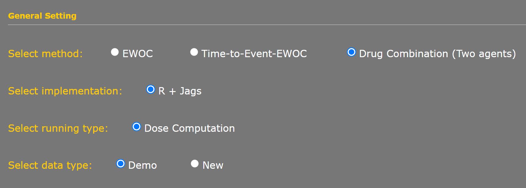
1. General Settings for Drug Combination Methods
Implementation is fixed as “R+Jags” which uses Markov Chain Monte Carlo sampling techniques.
Running Type is fixed for Dose Computation to calculate dosages for a series of consecutive patients based on previous data and design parameters set by the user.
Choosing “Demo” allows preset values to be entered as an example. “New” will allow you to work with a blank interface. “Previous Saved” is an option that can be chosen when loading parameters from a saved set.
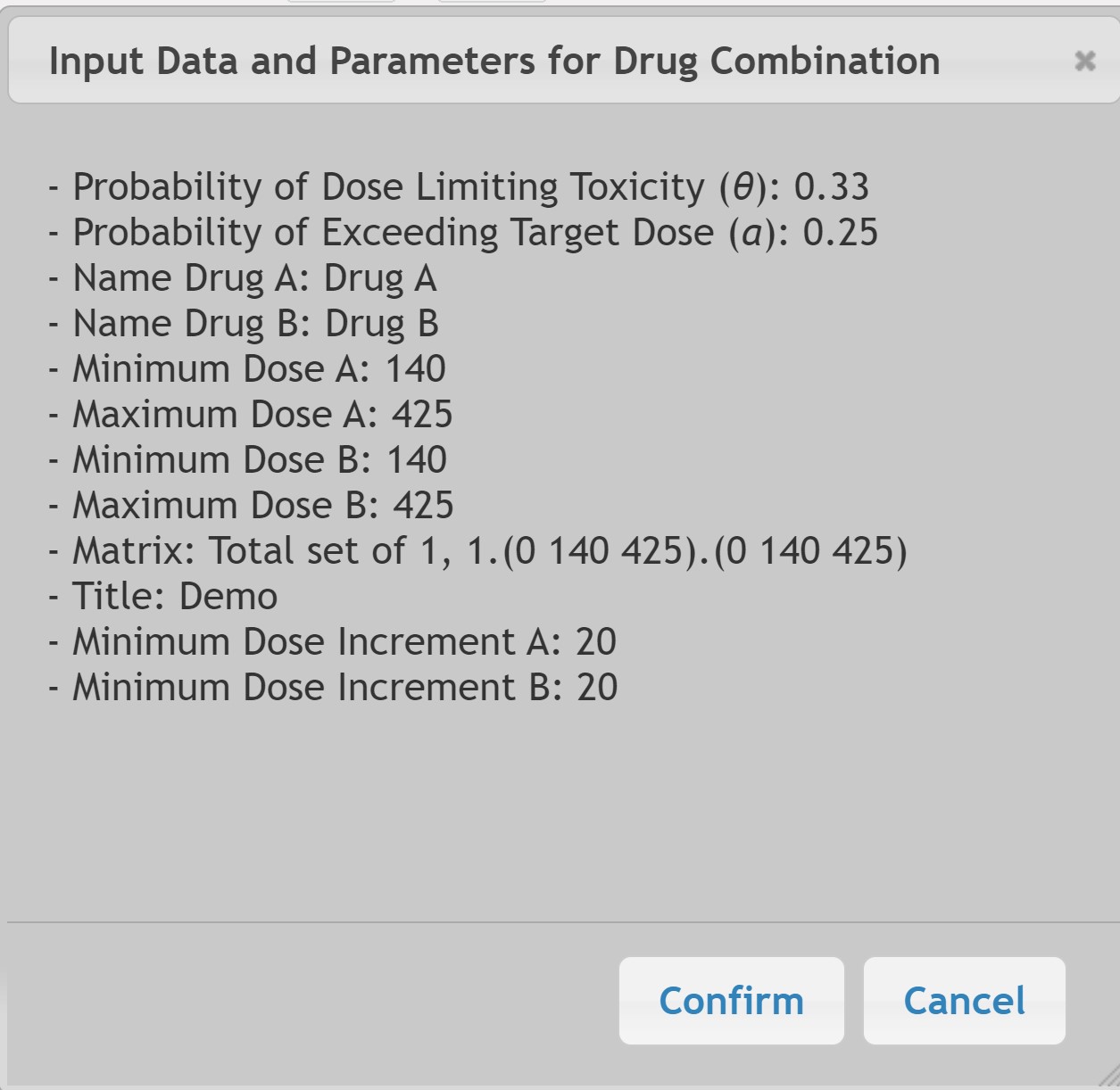
The Required Parameters are similar as described in Section V.2 but with the addition of parameters to allow for 2 drug combination, Indicated as Drug A and Drug B.
The Matrix Input assumes the first two patients will be enrolled at or above the lowest doses of both drugs and experienced no DLTs.
Note that Drug A and Drug B may have different Minimum and Maximum Dosage values.
The Optional Parameters allow for 2 drug combination with a maximum dose increment as a percent of the dose range. For example if the dose range is [10, 25], then a 20% increase would be 3 (15 x 0.2). Cohort size is fixed at two patients.
A basic understanding of Bayesian statistics is required for the input of these values. All four parameters must be set with a prior distribution by selecting “Plot prior density”.
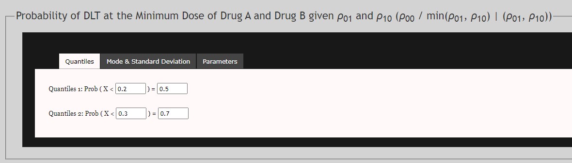
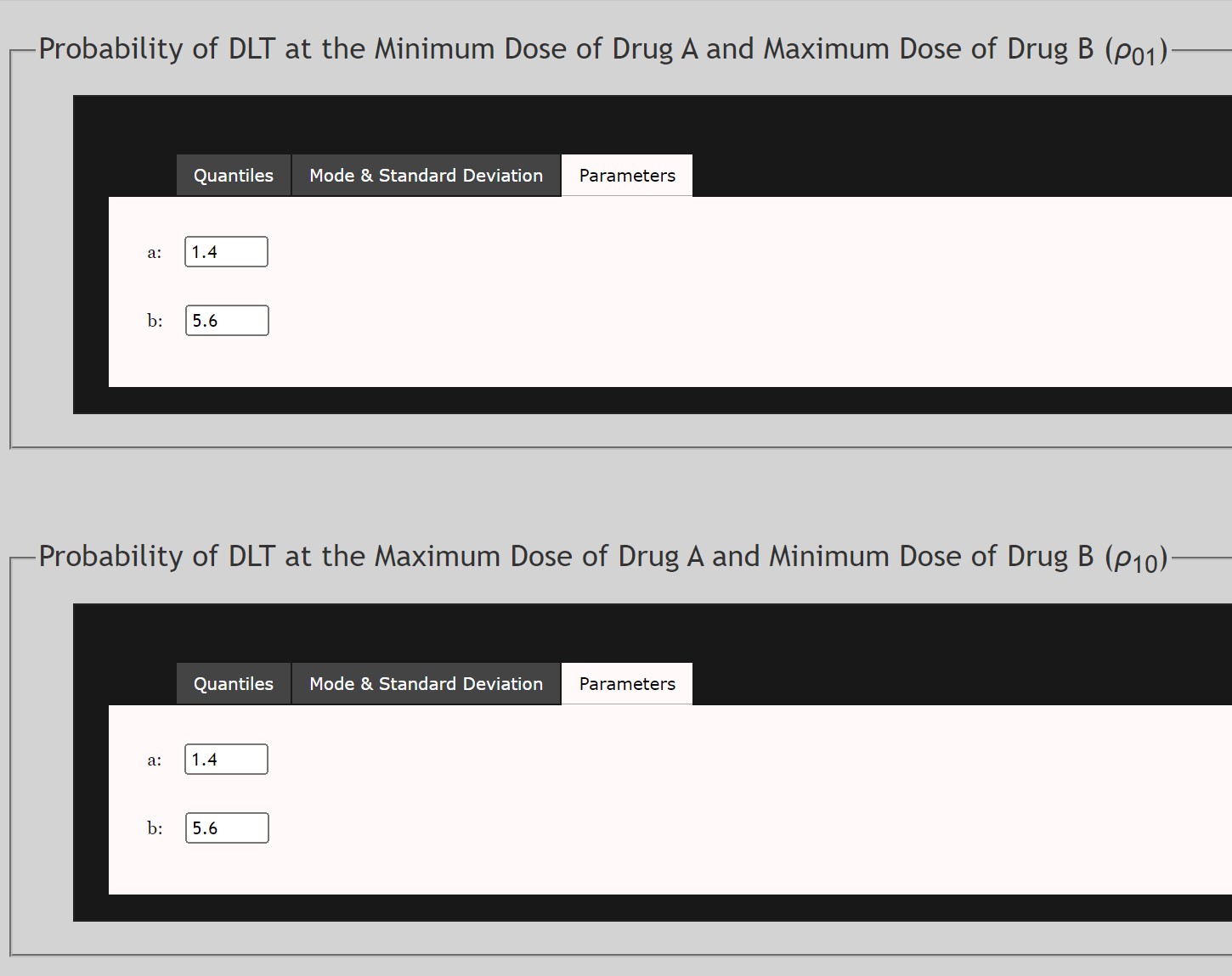
For the Prior Density of ρ01
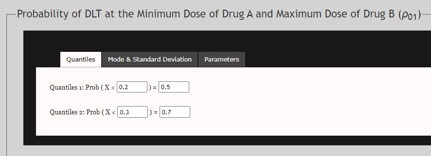
- This is the prior distribution of the probability of DLT at the minimum of Drug A and the maximum of Drug B. This prior follows a Beta Distribution. This data may be extrapolated based on other trials of Drug B used independently.
- Data may be input as either Quantiles, Mode and Standard Deviation, or α and β parameters of the Beta Distribution.
For the Prior Density of ρ10
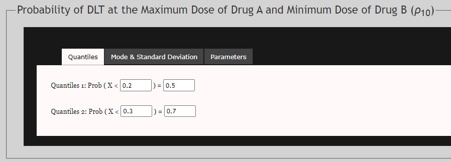
- This is the prior distribution of the probability of DLT at the maximum of Drug A and the minimum of Drug B. This prior follows a Beta Distribution. This data may be extrapolated based on other trials of Drug A used independently.
- Data may be input as either Quantiles, Mode and Standard Deviation, or α and β parameters of the Beta Distribution.
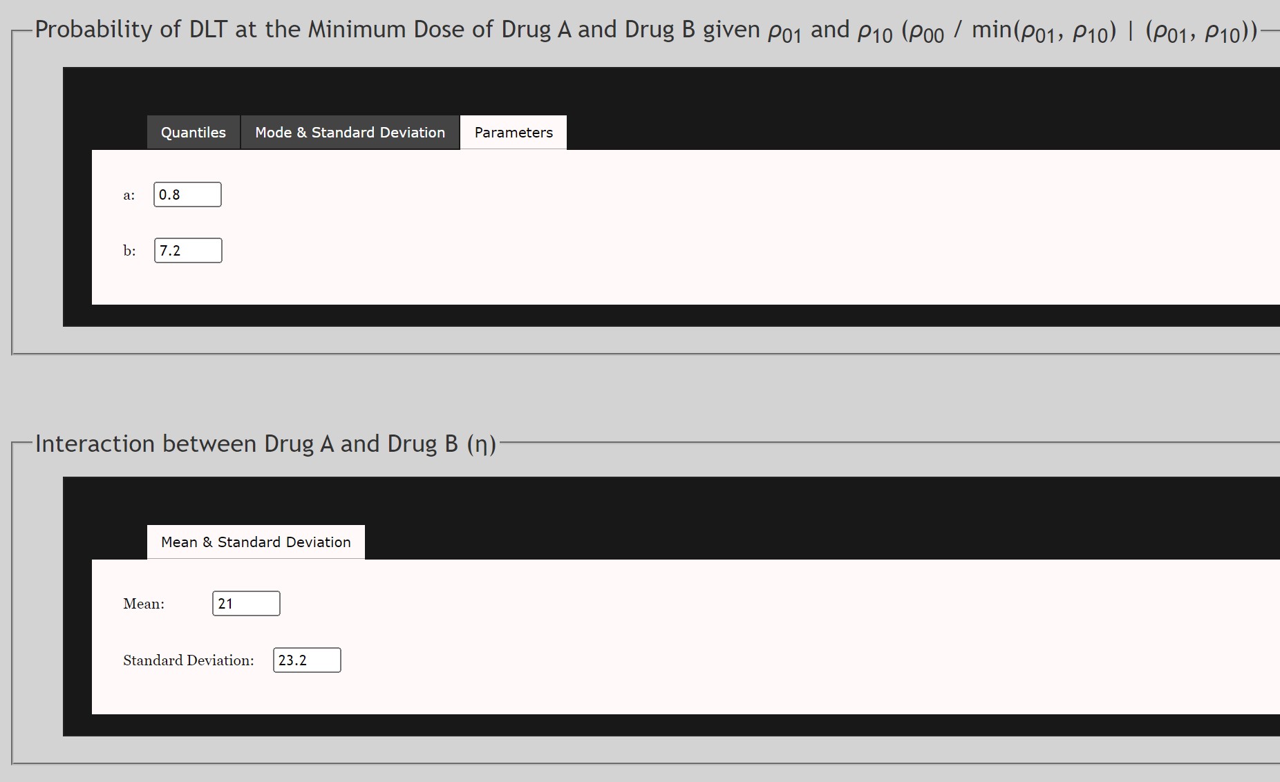
For the Prior Density of ρ00
- This is the prior distribution of the conditional probability of DLT at the minimum of both Drug A and Drug B. This prior follows a Beta Distribution. This data may be extrapolated based on other trials of Drug A or Drug B used independently. Note that
- Data may be input as either Quantiles, Mode and Standard Deviation, or α and β parameters of the Beta Distribution.
For the Prior Density of η
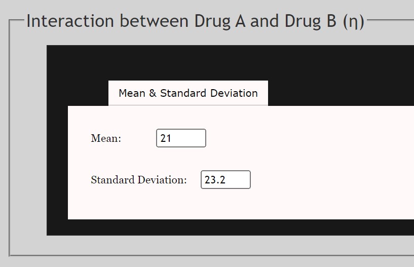
- This is the prior distribution of the interaction of ρ01 and ρ10 . This prior follows a Gamma Distribution. This data may be extrapolated based on other trials of Drug A used independently.
- Mean and Standard Deviation of the Gamma distribution are required.
- Select the
 button to set all parameters. PDF plots will appear of all prior densities. Review before proceeding.
Once all data has been input under each tab and the button is selected, a pop-up window will be displayed to allow review of parameters input. Select “Confirm” to compute next dose.
Two PDF files will be generated:
1) Report Results: This output window will be displayed for all results. It will include a section of Input Parameters and another section of Results which will include doses for the two patients.
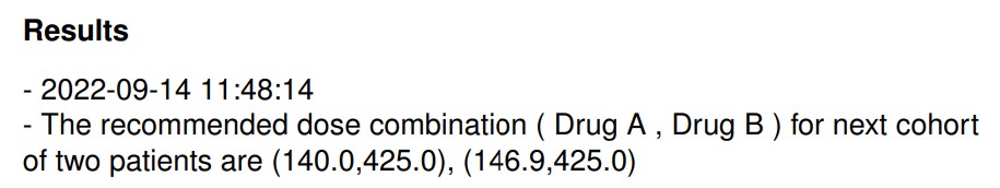
In example results above, Subject 3 will get Drug A at dose 140 and Drug B at 425. Subject 4 will get Drug A at 146.9 and Drug B at 425.
2) Marginal Posterior Probability Density Function: This plot is the marginal posterior probability density function of g (the MTD) and will change based on the data input under the "Priors" tab.
All results generated for a given project will be automatically saved and can be reviewed under the Results tab. For first time users, this tab will contain no data.
VI. Example Output - Dose Computations
Example 1 - EWOC Dose Computation with Discrete Doses (Open Bugs Implementation)
Note that this example uses the OpenBugs Implementation Option, although results should be similar under the Fortran option.

If the trial is based on a pre-specified set of discrete doses d1 < d2 < ... < dk, then assuming that di+1 - di = d for all i =2,..,k-1, set Xmin = d1 and Xmax = dk + d. The EWOC algorithm will treat the dose as continuous in the interval [d1, dk+d] and the recommended dose by EWOC is always rounded down to the nearest dose. For example, if the doses available in the trial are 20 ng/m2, increments then 20 ng/m2 should be entered in the Minimum Dose increments tent tab of the EWOC dialog box.
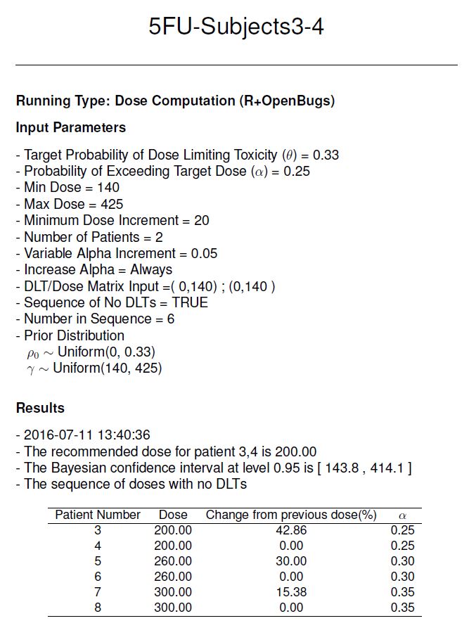
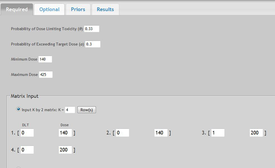
This is the example of the FU-trial described in Babb et al. (1998). The target probability of DLT is θ = 0.33 and the minimum and maximum dose levels allowable in the trial are Xmin =140 and Xmax = 425. A minimum dose increment of 20 is selected. Suppose we use a probability of exceeding the target dose α = 0.25 and a variable alpha increment of 0.05. Input values as illustrated below. The resulting EWOC-Dialog follows.
Alternatively, you could create and upload the following text file which would result in the same Matrix Input. Any text after the second value is not read in.

And under the "Optional" tab we would input the following:
Leaving the "Priors" option to a Uniform distribution:
Selecting "Calculate Next Dose" yields the following results:
Choose "Confirm" and the following results are displayed, which may be saved as a pdf.
You may use the Adobe Reader icons to save the .pdf to your computer or to print.
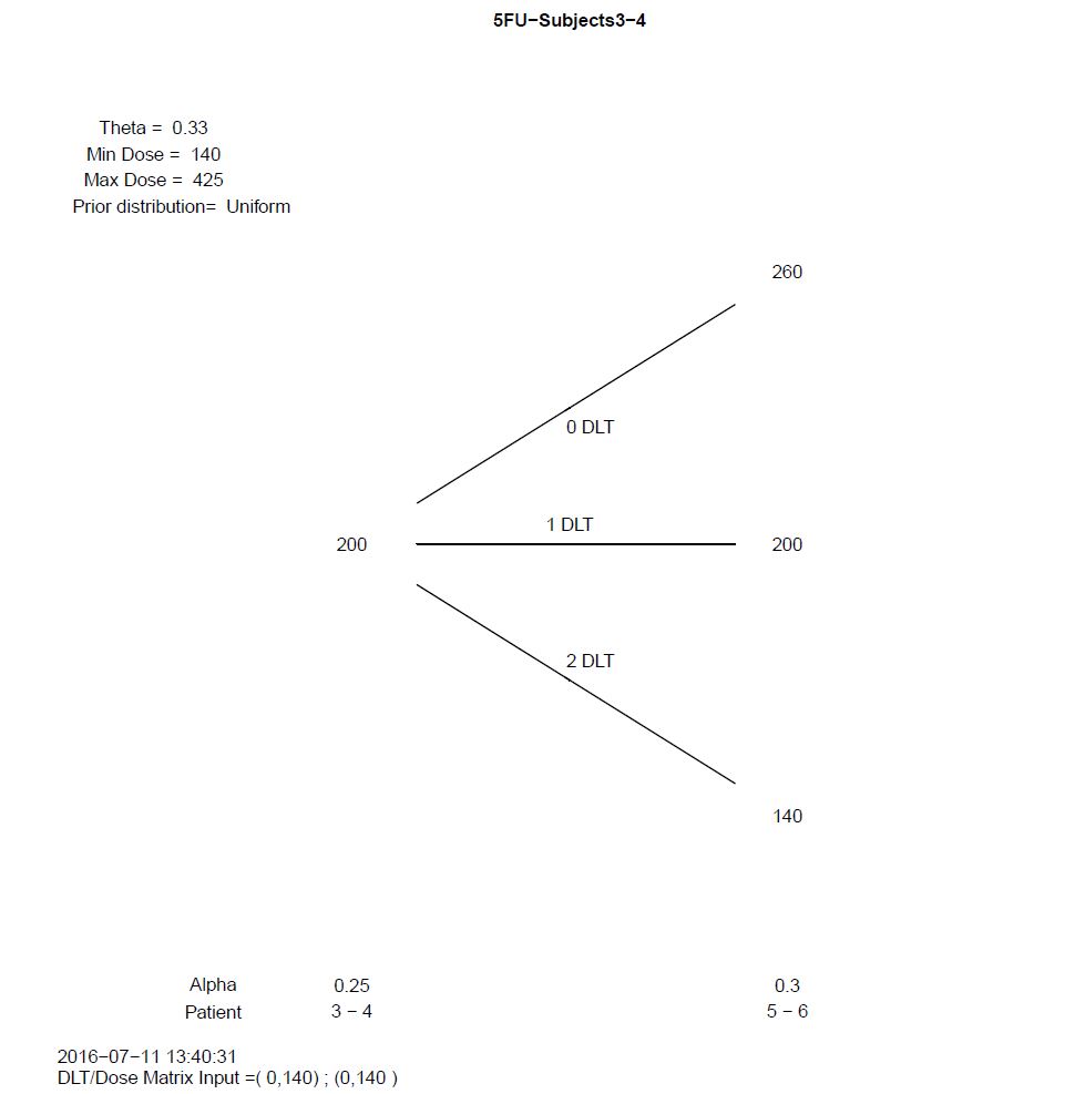
The "Tree of Doses" results are displayed since that option was selected:
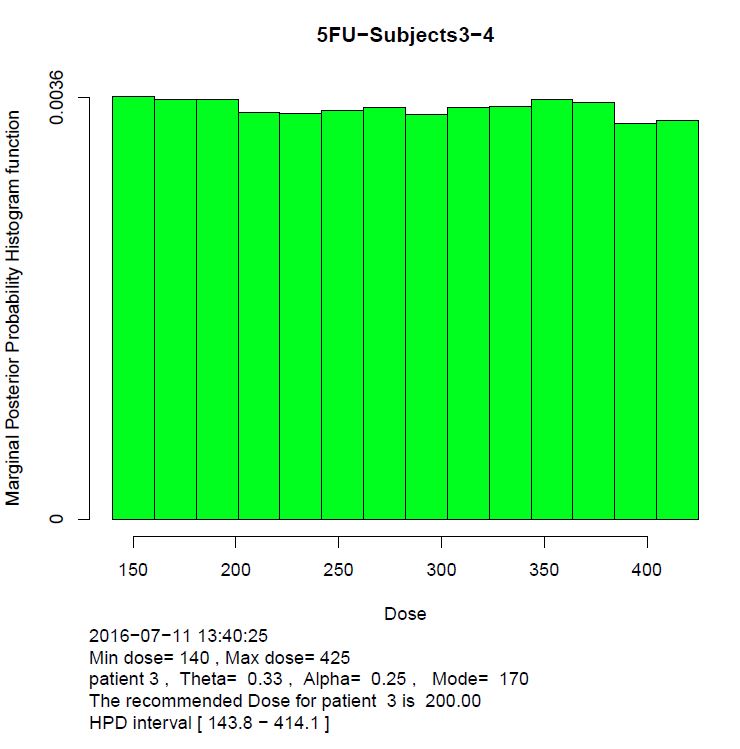
The "Posterior Distribution of Target Dose Plot" is also displayed should that option have been selected under the "Optional" tab.
Note that because this was run with the "OpenBugs" Implementation method, which utilizes sampling, the posterior distribution is represented by a histogram.
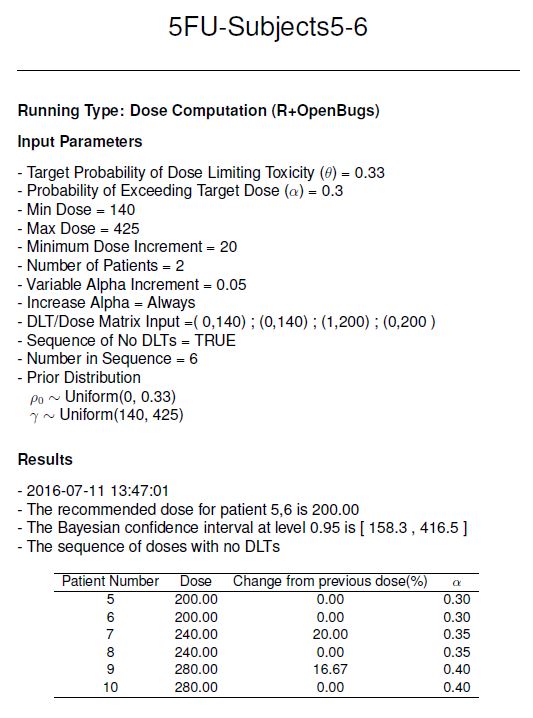
According to these results, Subjects 3 and 4 should both receive 200 ng/m2. Let’s suppose Subject 3 experienced a DLT, and Subject 4 did not.
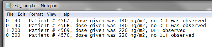
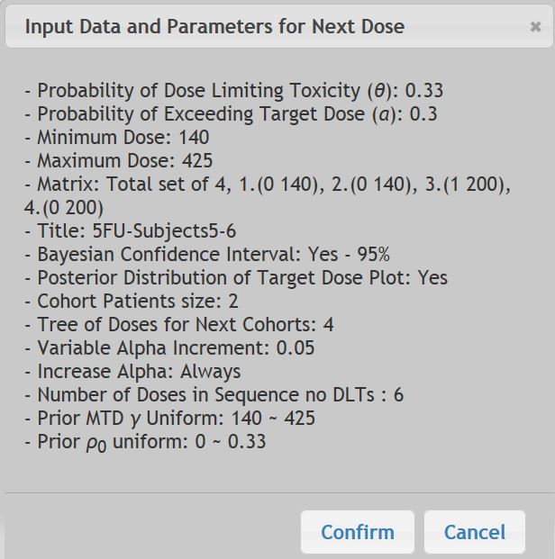
To calculate the dosing for Subjects 5 and 6, we return to the "Required" Tab. The alpha level would be increased now to 0.3 under this scenario. Under the Matrix Input the following data would be input:
Or if you wished to upload a Data File, for example:
The data entered under the "Optional" tab will remain the same as above, with Uniform Priors. After selecting the "Calculate Next Dose" button, the following Confirmation window would appear followed by results listed below:
Marginal posterior distribution plot
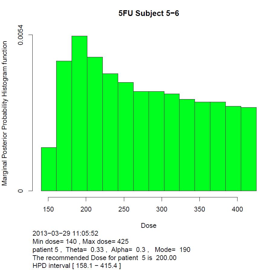
The Marginal posterior distribution (y-axis) versus Dose (x-axis) plot. It can be viewed as a probabilistic summary about the Target dose and conveys all the information accumulated from the previous patients. The first line at the top displays the title. Below the histogram, is printed the date and time stamp, Xmin and Xmax, patient number, the Probability of dose limiting toxicity (θ) and the Probability of exceeding the Target dose (α). The EWOC recommended dose and the 95% HPD interval is also reported. The fundamental property of the EWOC recommended dose is that the area under the curve between it and Xmin is the chosen Probability of exceeding the Target dose (α).
Continuing in this example where the first two patients are given dose level 140, and none of them had DLT, while 1 patient dosed at the 200 level experienced a DLT. Suppose we want to have a tree of doses for the next four cohorts of 2 patients. The tree displays the recommended doses for the next four cohorts considering all possible outcomes.
In computing the dosing schema, when a sequence of DLTs are observed at Xmin, and especially if the variable alpha is used, EWOC may produce incoherent results. Recall that EWOC assumes no DLTs can occur at Xmin. When this assumption is violated and alpha is incremented, the resulting dosing estimates may be incoherent. In practice, if a DLT were to be observed at Xmin, the study should be halted and re-designed.
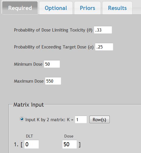
2. Example 2 - Dose Computation with Continuous Dosing Schema (Fortran Implementation)
While either Fortran or OpenBugs can be used in any example, here we will demonstrate using the Fortran method.

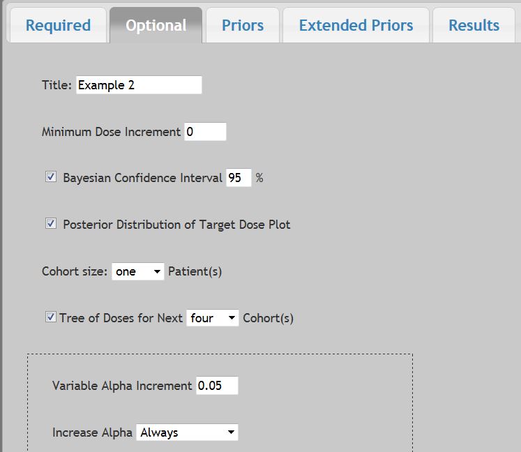
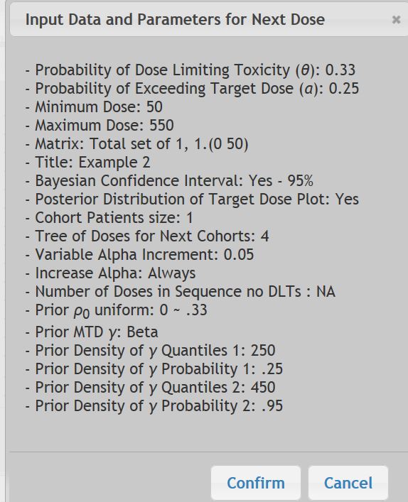
Suppose you want to design a phase I trial where the target probability of DLT is θ = 0.33 and the doses available in the trial are unlimited, with a desired dose range of Xmin = 50 ng and Xmax = 550 ng. The first patient in the trial will be given dose 50 ng and you want to treat one patient at a time. Suppose we use a probability of exceeding the target dose α = 0.25 and a variable alpha increment of 0.05. Suppose we want the tree of doses for the first 4 patients. And we assume a Beta distribution for γ.
The corresponding input would be:
And the Optional input would be:
And let’s assume we believe the MTD has a prior Beta distribution with a 25% probability of being <250 ng but 95% probability of <450 ng.
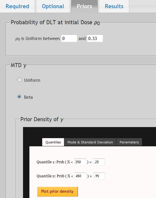
Selecting the "Plot Prior Density" we get:
Once you select "Calculate Next Dose" the Input Data window will show:
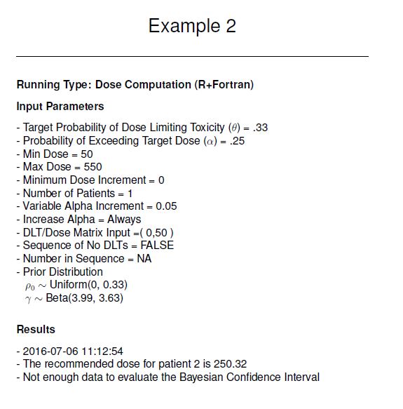
The Results would be:
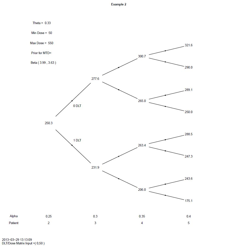
With the resulting Tree of Doses:
And the following Posterior Distribution of the MTD (γ):
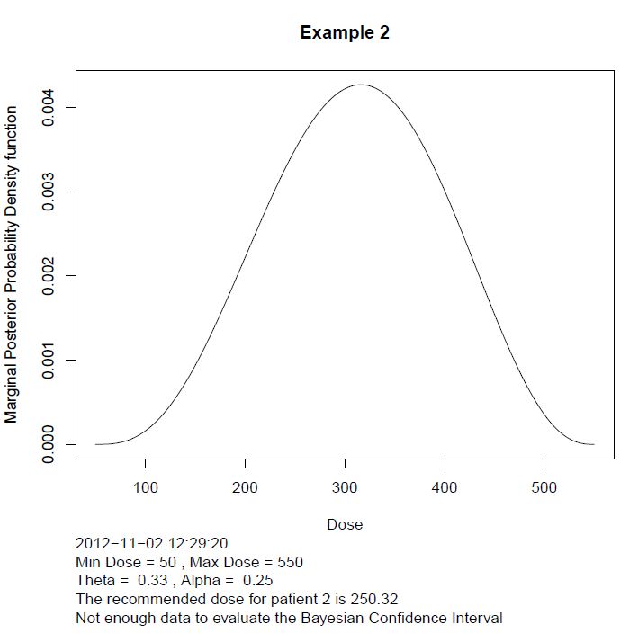
Note that because the implementation was performed with Fortran, the resulting posterior distribution is a smooth function.
3. Example 3 - Time-to-Event Dose Computation
Models to estimate the MTD that use the exact time when a DLT occurs are expected to be more precise than those where the variable of interest is categorized as only present or absent. Time-to-Event EWOC is also advantageous to allow enrollment of new subjects when the determination of DLT has yet to be resolved from previous subjects. See Tighiouart et al, 2014 for a detailed discussion of the methodology.

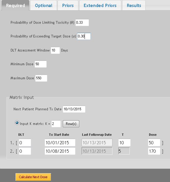
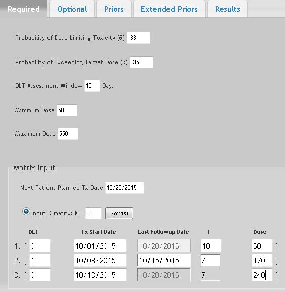
In the following example for a Phase I trial, the target probability of DLT is θ = 0.33 and the doses available in the trial are available only in 5 ng increments, with a desired dose range of Xmin = 50 ng and Xmax = 550 ng. The first patient in the trial will be given dose 50 ng and you have a 10-day window to observe for DLT. Suppose we use a probability of exceeding the target dose α = 0.25 with a variable alpha increment of 0.05, and a Uniform distribution for g.
Subject 1 was enrolled on 10-1-2015 at 50ng with and no DLT was observed.
Subject 2 was enrolled on 10-8-2015 at 170ng with θ = 0.25 and so far no DLT has been observed.
Subject 3 is ready on today's date of 10-13-2015, and we increase α = 0.30 per study guidelines
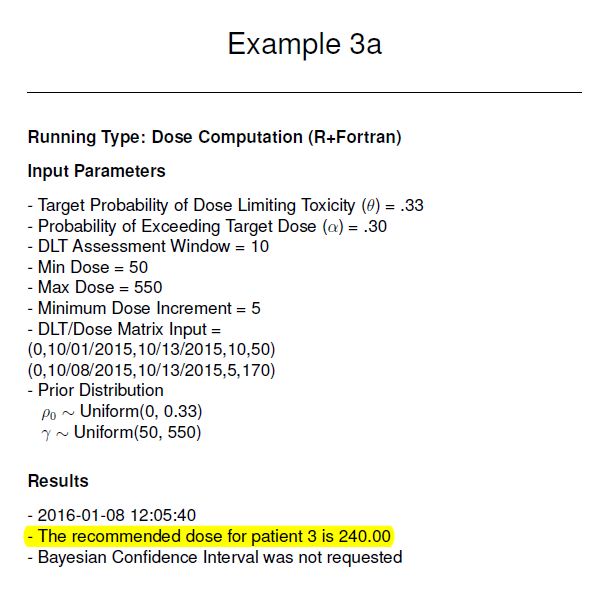
After selecting the "Calculate Next Dose" button, a pop-up window will appear to confirm the data input:
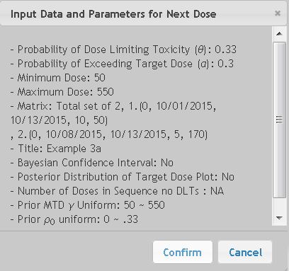
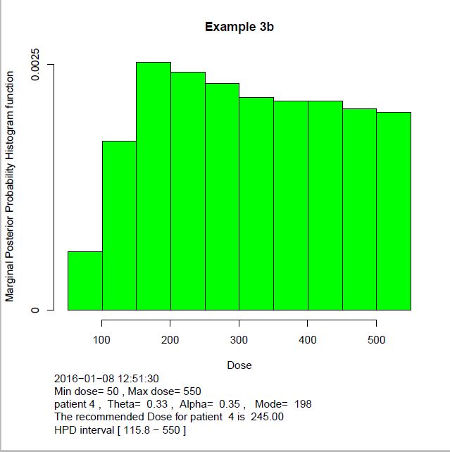
Select "Confirm" on the pop-up window will generate a PDF report which will indicate Subject 3 should be given 240ng:
Now suppose after Subject 3 was enrolled, Subject 2 had a DLT on 10-15-2015, and we are now ready to enroll Subject 4. The input data should now be:
Subject 1 was enrolled on 10-1-2015 at 50ng with and no DLT was observed.
Subject 2 was enrolled on 10-8-2015 at 170ng with DLT on 10-15-2015.
Subject 3 was enrolled on 10-13-2015 at 240ng with no DLT observed to date.
Subject 4 is ready to enroll today on 10-20-2015 and we increase α = 0.35 per study guidelines
The resulting PDF file reports the recommended dose for Subject 4:

And (if requested) the posterior distribution is also generated:
4. Example 4 - Two Drug Combination Studies
Phase I dose finding trials of two-drug combination therapy traditionally are designed to estimate the MTD of a single drug for a given fixed dosage of the other agent. While results may provide a final safe dose for the combination, the therapeutic effect may be sub-optimal. EWOC can be used for estimating the MTD of two drugs in combination.
In this module EWOC assumes:
- Each drug combination is tested in a cohort of 2 subjects.
- The first cohort of 2 subjects receive the same drug combination dosages of the two drugs at or above the minimum dose of each drug as decided by the study protocol.
- That DLT data are available on each prior cohort of 2 subjects before escalating to next dose combination.
(See Tighiouart et al, 2017, and Tighiouart 2019 for more detailed explanation.)

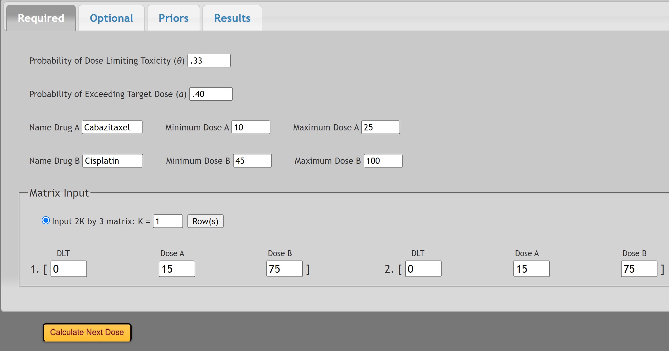
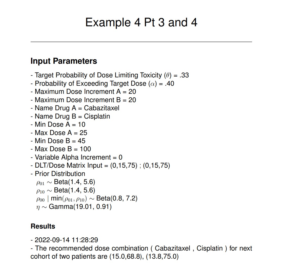
In the following example for a Phase I two drug trial, the target probability of DLT for the combination of Drug A with Drug B is θ=0.33. Drug A (Cabazitaxel) can be given in a range of 10 to 25 mg/m2 and Drug B (Cisplatin) can be given in a range of 45 to 100 mg/m2:
The first two subjects were treated per protocol with Cabazitaxel at a dose of 15mg/m2 and Cisplatin at 75 mg/m2 and no DLTs were observed.
We will use a probability of exceeding the target dose of α=0.40 at study start with a variable alpha increment of 0.05 only if no DLT is observed in the prior cohort of subjects. Note that the alpha value will need to be input as 0.40, 0.45, and 0.50 with each sequential patient cohort according to the prior sequence of DLTs observed.
To compute the dosing for Patients 3 and 4, the input under the Required tab is:
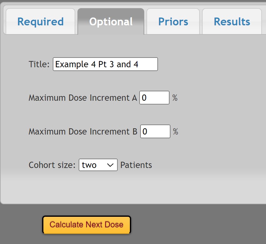
And the input under the Optional tab:
For this example, informative priors were selected for the probability of DLT with the parameters of:
With a vague prior for the interaction term:
After selecting and  then
then  :
:

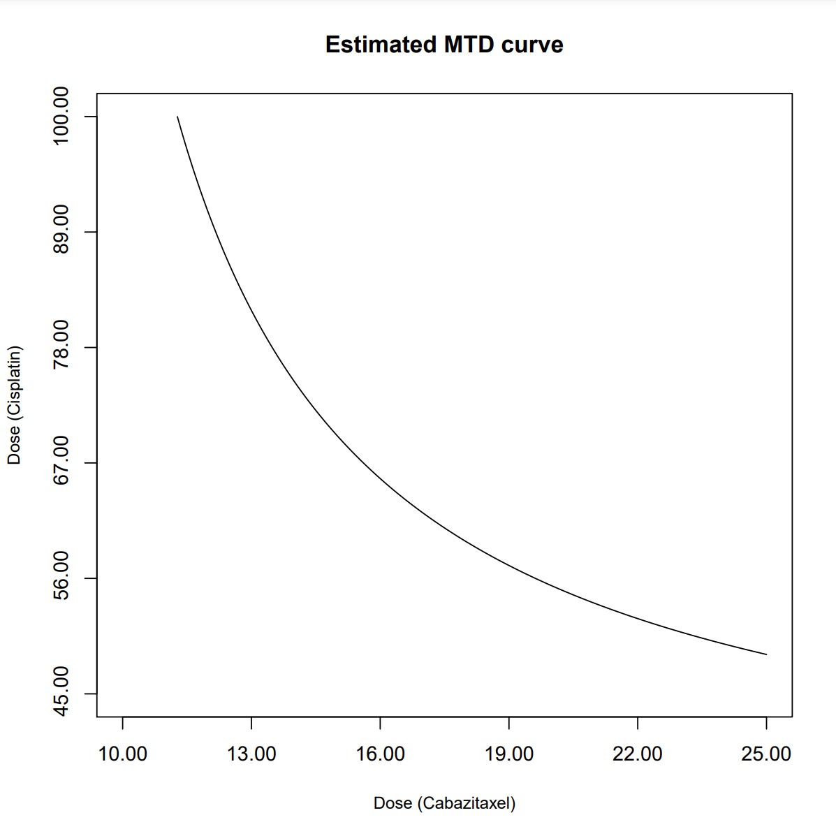
The resulting PDF files indicate the dosing for subjects (3, 4) is (15.0, 68.8) and (13.8, 75.0), with the corresponding MTD curve:
VII. Running EWOC - Trial Simulation Mode
This mode allows you to simulate trials and generate design operating characteristics for either a continuous dose or a discrete set of increasing doses di, i=1, ... ,k.
For a continuous dose, the user specifies the minimum and maximum allowable dose, the value of the true MTD γtrue , and the probability of DLT at the minimum dose ρ0.
For a discrete set of k doses, the user can either specify the probability of DLT at each dose level or specify the probability of DLT at Xmin and the dose level j such that dj is the true MTD, γtrue. Let d0 = Xmin, dk+1 = Xmax. Here, we assume that the support of the MTD is [Xmin, Xmax], Xmin < d1 < d2 < ... <dk < Xmax, and di+1 - di is constant for all i = 0, ... ,k.
DLT responses are generated from the true logistic model. Trial Simulations will only run under the R + Fortran implementation setting.
General Settings - Select Data Type
Choosing "Demo" allows preset values to be entered as an example. "New" will allow you to work with a blank interface. "Previous Saved" is an option that can be chosen when loading parameters from a saved set.
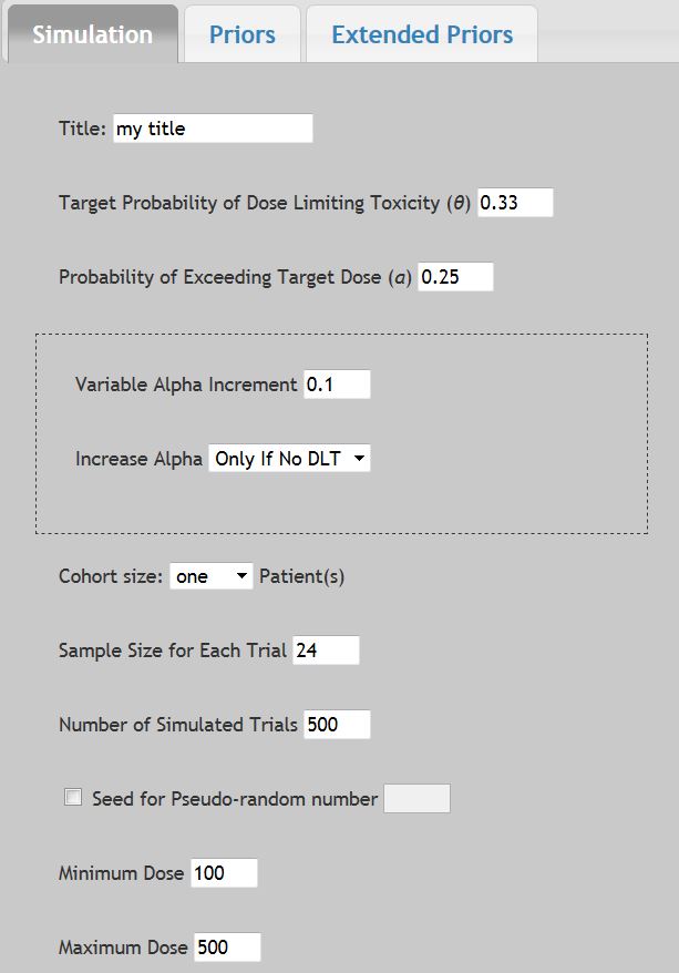
Title
Up to 100 characters can be used to label all output and printable reports.
Target Probability of Dose Limiting Toxicity (θ)
This is the proportion of patients expected to experience a medically unacceptable, dose-limiting toxicity (DLT) if the Target dose (or maximum tolerated dose, MTD) is administered. Its value, generally between 0.1 and 0.5, depends on the nature of the DLT. It would be set relatively high when the DLT is a transient, correctable or non-fatal condition, and low when it is lethal or life threatening. In the dialog window above, the default value is θ = 0.33.
Probability of Exceeding Target Dose (α)
As when running in the Dose Computation Mode, this is the probability that the dose selected by EWOC is higher than the Target dose. Low values make the escalation cautious, high values cause larger steps. In the beginning of a trial, there is a higher level of uncertainty about the Target dose. Consequently, at the onset of a phase I trial, the probability of exceeding the Target dose is typically set to a low value (e.g., 0.25) in order to minimize the possibility of harming patients by administering doses much greater than the Target dose. In the dialog window above, the default value is α = 0.25. As the trial progresses, uncertainty about the Target dose declines and the likelihood of administering a dose considerably higher than the Target dose decreases. Thus, one should consider gradually increasing α during the course of the trial. When the probability of exceeding the Target dose is set to the maximum value of 0.50, it implies that under dosing a patient (treating with a dose lower than the Target dose) is just as bad as overdosing.
Variable Alpha Increment
The probability of exceeding target dose (α) can be gradually increased during the course of the trial to meet the need of a relatively higher probability of exceeding target dose as the trial progresses and the uncertainty about the target dose declines. The cumulative value for alpha will stop once α = 0.5 (the maximum allowable value). You may also choose to increase the alpha value "Always" or "Only If No DLT" from the drop down menu. When Variable Alpha Increment input value is set to 0 the "Increase Alpha" drop down will default to the "Always" selection, indicating the alpha value will remain constant during the course of the trial.
Cohort Size
This option allows you to design a trial with cohorts of p patients at each dose level, p =1, 2, 3. The default is one patient. To select either two or three patients, click the right corner for the drop-down box, and then select either two or three to make the selection, which will then be highlighted.
Sample Size for Each Trial
This allows you to set the maximum number of subjects for each simulation. Larger subject numbers will increase the simulation run times. The default value is set to 24. The allowable range is 1 to 99.
Number of Simulated Trials
This allows you to set the number of simulations run. Larger simulations will take longer computing time. The default value is set to 500. The allowable range is 1 to 10,000.
Seed for Pseudo-Random Number
This allows you to set a seed for computations. This will help fix results to be consistent between runs. Leaving this box unchecked allows for a Random Seed. When selected, the default value is set to 1. The allowable range is 1 to 100.
Minimum Dose
This is the lower bound Xmin of the support of the MTD γ. The dose to be given to the first patient in the trial is always greater than or equal to Xmin. Note that the dose given to the first cohort of patients is not necessarily equal to Xmin but there must be strong evidence that it is a safe dose. EWOC will never assign doses below Xmin. In the dialog window above, the default value is Xmin = 140. The allowable range is 0 to 500.
Maximum Dose
This is the upper bound Xmax of the support of the MTD γ. The highest allowable dose in the trial must be less than or equal to Xmax. EWOC will never assign doses above Xmax. In the dialog window above, the default value is Xmax = 425. Values must be greater than 0.
2. Scenario Setup for Continuous Doses
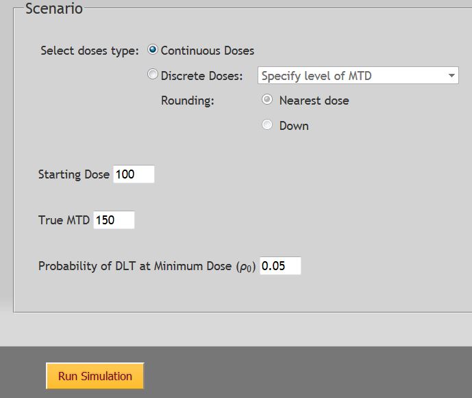
Starting Dose
Enter the first dose for the first patient. Based on the protocol design, it may be of use to start at any point between the Minimum and Maximum doses. It may not be less than or greater than the values entered above for Minimum and Maximum doses.
True MTD
Enter the value to assign as the True MTD under the proposed scenario. It must be between the proposed Minimum and Maximum Doses. The default value is set to 150.
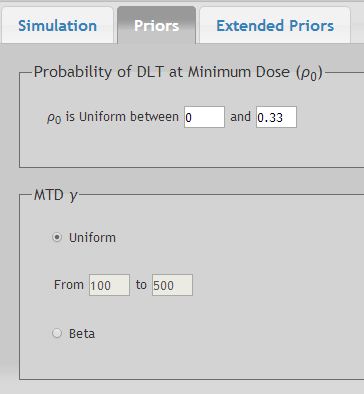
Probability of DLT at Minimum Dose (ρ0)
This value is the probability of dose limiting toxicity at the minimum dose. The value entered must be less than the Probability of Dose Limiting Toxicity (θ) entered above.
3. Scenario Setup for Discrete Doses - Specifying the Level of MTD

Rounding
There are two options for rounding and the choice depends on the experimental design. "Nearest Dose" will allow for rounding to be up or down, while selecting "Down" will always round to the lesser value. Rounding down is sometimes preferred to increase patient safety.
Starting Dose
Enter the first dose level for the first patient. This value must be a whole integer. The minimum value is 1 and the maximum allowable value is the total number of discrete dose levels entered below. Based on the protocol design, it may be of use to start at any point between the Minimum and Maximum doses levels.
Number of Discrete Dose Levels
Enter in the total number of doses planned for study. It is assumed the doses will be equally spaced in the modeling on a standardized scale. The value must be an integer between 3 to 20 doses.
Dose level of True MTD
Enter an integer which corresponds to the dose number which is to be assigned as the true MTD in the simulation scenario. For example, if there are 7 discrete dose levels and it is assumed the true MTD dose is level 4 then here enter the number 4. The minimum value is 1 with a maximum value equal to the value of the total number of discrete dose levels entered above.
Probability of DLT: (ρ0)
For the purposes of mathematical modeling, discrete doses are assumed to be equally spaced inside the interval [0, 1]. Here, ρ0 is the probability of DLT at dose d0 as defined at the beginning of Section VIII. The allowable range is any value greater than zero that is less than the Target Probability of DLT entered previously. A value of 0.05 is recommended.
4. Scenario Setup for Discrete Doses - Probability of DLT at Dose Levels
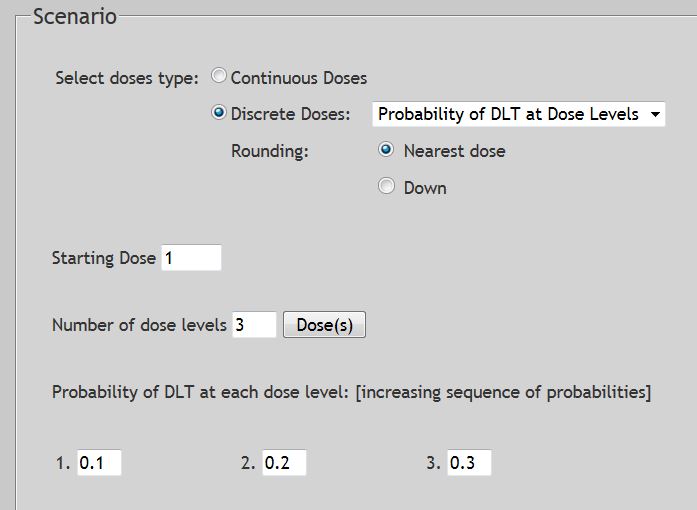
Rounding
There are two options for rounding and the choice depends on the experimental design. "Nearest Dose" will allow for rounding to be up or down, while selecting "Down" will always round to the lesser value. Rounding down is sometimes preferred to increase patient safety.
Starting Dose
Enter the first dose level for the first patient. This value must be a whole integer. The minimum value is 1 and the maximum allowable value is the total number of discrete dose levels entered below. Based on the protocol design, it may be of use to start at any point between the Minimum and Maximum doses levels.
Number Dose Levels
For the purposes of mathematical modeling, discrete doses are assumed to be equally spaced inside the interval [0, 1]. Here, ρ0 is the theoretical risk of DLT at Xmin, a dose below the smallest available discrete dose level in the trial. The allowable range is any positive value that is less than the Target Probability of DLT entered previously.
Probability of Each Dose Level
Enter in the probability of DLT for each of the corresponding doses. The simulation modeling assumes increasing risk with increasing dosing. Values must be between 0 and 1 and successively increasing.
5. Simulation Setup - Priors & Extended Priors Tabs
We do not recommend changing the defaults for the prior distributions unless you have a basic understanding of Bayesian statistics.
For the Probability of DLT at Minimum Dose ρ0
The default is the uniform distribution between zero and θ, the probability of dose limiting toxicity at the Target dose. The upper limit field changes automatically as θ does. To make them different from each other, change the upper limit field AFTER each change made for θ under the Simulation tab.
For the Maximum Tolerated Dose (γ) dose
The default for the MTD is the uniform distribution between Xmin and Xmax. Alternatively, a Beta distribution can be selected. See Pages 13-14 for detailed explanation.
Extended Priors
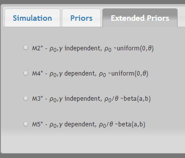
Additional extended priors are available for more advanced modeling using distributions as described in Tighiouart et al 2005. See Pages 15-16 for detailed explanation.
6. Running Simulation - Results
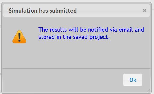
Once the "Run Simulation" button is selected, the following window will appear. Choose "Confirm" to continue. A second window will pop up once the Simulation is submitted informing that an email notification will go out via email when the results are ready. Trials will be simulated sampling from a logistic distribution that passes by the points (Xmin, ρ0) and (α, θ).
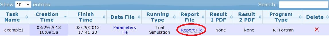
The simulation may take several hours to complete. Once the simulation is finished, click on the link sent via email to return to the EWOC workspace. After your login, choose "Saved Project" then "Select" the project you wish to return to. Your results will appear under the following "Tasks" sub-menu.
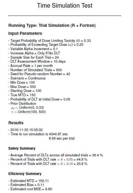
Choose "Report File" to see the Simulation Results.
The resulting Report File will summarize the input parameters and report the results of the simulation.
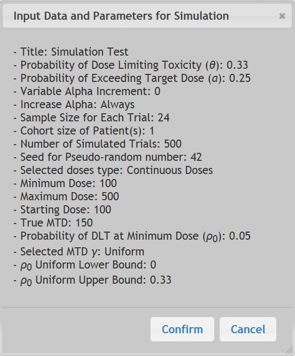
In this example, we want to design a cancer phase I trial with a target probability of DLT θ = 0.33, and a fixed probability of exceeding the target dose α = 0.25. A maximum of 24 patients will be enrolled to the trial. Dose levels are continuous between 100 and 500 mg and the first patient receives the dose 100 mg. We want to obtain design operating characteristics by simulating 500 trials assuming that the true MTD is 150 and the probability of DLT at the lowest possible dose is 0.05. Note that the seed for the random number generator was set to 42.
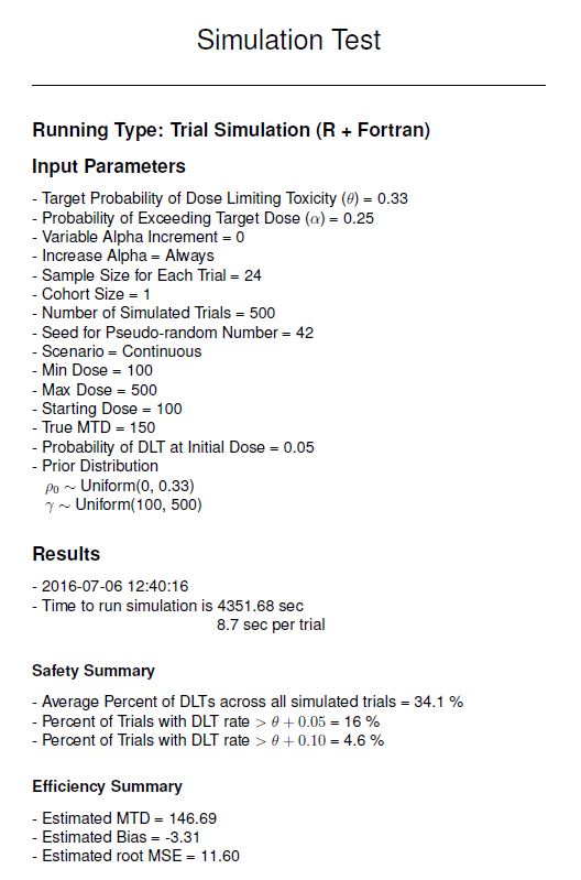
Under "Safety Summary" we see there were on average 34.1% DLT’s experienced across all 500 simulated trials, which is close to the target probability of DLT was set at 0.33. We see also that 16% of all simulation trials had a DLT rate greater than 0.38 (θ + 0.05).
Under "Efficiency Summary" the output is calculated as follows:
Estimated MTD is defined as: 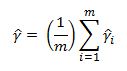
where ![]() is the estimated MTD of the i-th trial as well as the dose recommended for the n+1 patient in the i-th trial, and m is the number of trials simulated.
is the estimated MTD of the i-th trial as well as the dose recommended for the n+1 patient in the i-th trial, and m is the number of trials simulated.
Estimated Bias is defined as: ![]()
The Estimated root MSE is defined as: 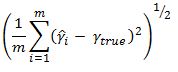
The table included at the bottom gives the percent of patients who were Under dosed, Optimally dosed, or Over dosed, depending on the Tolerance window around the Optimal dose value. Note that the shape of the distribution is unknown and typically asymmetrical.
VIII. Running Time-to-Event-EWOC – Trial Simulation Mode
One limitation of EWOC is that the toxicity outcome is coded as binary as the presence or absence of DLT. However, in some dose finding studies, the observation time to resolve a subject's outcome may be very long. Under the original EWOC design rather than delaying enrolment of a new subject while waiting for the previous subject's results, a new subject would simply be assigned the same dose until additional data could be collected. This limitation motivated the development of models to estimate the MTD that take into account the time subjects are under observation.
Of note, this modeling assumes that should the DLT status of the previously enrolled subject is not known when a new subject is ready to start, then the longer the time the previous subject goes without experiencing a DLT, the higher the recommended dosage would be for the new subject. Correspondingly, should a previous subject experience a DLT shortly after drug administration, then the next dose computed would be lower than if the previous DLT had happened later. We assume the risk of DLT for any given dose follows a Cox proportional hazards model.
This mode allows you to simulate Time-to-Event trials and generate design operating characteristics for either a continuous dose or a discrete set of increasing doses di, i=1,…,k.
For a continuous dose, the user specifies the minimum and maximum allowable dose, the value of the true MTD γtrue, and the probability of DLT at the minimum dose ρ0.
For a discrete set of k doses, the user can either specify the probability of DLT at each dose level or specify the probability of DLT at the initial dose and the dose level j such that dj is the true MTD, γtrue. Let do = Xmin, dk+1 = Xmax. Here, we assume that the support of the MTD is [Xmin, Xmax], Xmin < d1 < d2 <… < dk < Xmax, and di+1 – di is constant for all i = 0, …,k.
We assume that patients arrive to the trial according to a time homogeneous Poison process and the time to DLT is generated from the true model with a baseline exponential hazard function. If a DLT time is > τ, then this time is right censored at τ .. Trial Simulation will only run under the R + Fortran implementation setting.
(See Tighiouart et al, 2014, for more detailed explanation.)
General Settings - Select Data Type
Choosing "Demo" allows preset values to be entered as an example. "New" will allow you to work with a blank interface. "Previous Saved" is an option that can be chosen when loading parameters from a saved set.
All Simulation, Scenario, Priors, and Extend Prior Parameters are the same as described in Section VIII, with the following changes to allow for the observation time to resolve a DLT.
Note that it is assumed the cohort size is always 1, and that no two subjects will be enrolled on the exact same date.
DLT Assessment Window
This is the number of days the study protocol allows for a DLT to be resolved. The observation window is defined as (0,τ].
Accrual Rate
Enter the proposed number of patients to enroll for treatment per month. This will automatically define the rate of the time homogeneous Poisson process.
2. Running Time-to-Event Simulation - Results
Once the "Run Simulation" button is selected, the following window will appear. Choose "Confirm" to continue. A second window will pop up once the Simulation is submitted informing that an email notification will go out via email when the results are ready.
The simulation may take several hours to complete. Once the simulation is finished, click on the link sent via email to return to the EWOC workspace. After your login, choose "Saved Project" then "Select" the project you wish to return to. Your results will appear under the following "Tasks" sub-menu.
Choose "Report File" to see the Simulation Results.
The resulting PDF Report File will summarize the input parameters and report the results of the simulation.
In this example, we want to design a cancer phase I trial with a target probability of DLT θ = 0.33, and an initial probability of exceeding the target dose α = 0.05, with increases in alpha of 0.1 for every patient that does not experience a DLT. A maximum of 24 patients will be enrolled to the trial. It will take 10 days to resolve if a patient has experienced a DLT and we assume enrollment of 6 subject a month. Dose levels are continuous between 100 and 500 mg and the first patient receives the dose 100 mg. We want to obtain design operating characteristics by simulating 500 trials assuming that the true MTD is 150. Note that the seed for the random number generator was set to 5.
Under "Safety Summary" we see there were on average 37.7% DLT's experienced across all 500 simulated trials, which is close to the target probability of DLT was set at 0.33. We see also that 38.8% of all simulation trials had a DLT rate greater than 0.38 (θ + 0.05).
Under "Efficiency Summary" the output is calculated as follows:
Estimated MTD is defined as:
where ![]() is the estimated MTD of the i-th trial as well as the dose recommended for the n+1 patient in the i-th trial, and m is the number of trials simulated.
is the estimated MTD of the i-th trial as well as the dose recommended for the n+1 patient in the i-th trial, and m is the number of trials simulated.
Estimated Bias is defined as: ![]()
The Estimated root MSE is defined as:
The table included at the bottom gives the percent of patients who were Under dosed, Optimally dosed, or Over dosed, depending on the Tolerance window around the Optimal dose value. Note that the shape of the distribution is unknown and typically asymmetrical.
1. EWOC Mathematical Formulation
A detailed description of the mathematical concepts underlying EWOC can be found at:
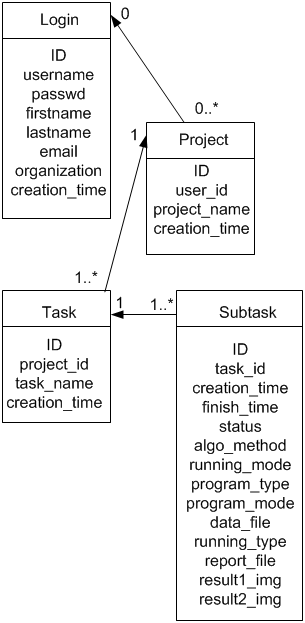
2. WEB-EWOC High Level Systems Architecture
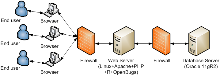
There are 6 tables in the database to store user’s profile, project, task, subtask, and parameters information. Here we provide the Entity-Relationship diagram of core tables of the system.
- Babb J, Rogatko A, Zacks S. 1998. Cancer phase I clinical trials: efficient dose escalation with overdose control. Stat. Med. 17:1103-1120.
- Babb JS, Rogatko A. 2001. Patient specific dosing in a cancer phase I clinical trial. Stat. Med. 20:2079-2090.
- Babb JS, Rogatko A. 2004. Bayesian Methods for Cancer Phase I Clinical Trials. In: Advances in Clinical Trial Biostatistics, edited by Nancy Geller, New York, Marcel Dekker, pp. 1-40.
- Cheng J, Babb JS, Langer C, Aamdal S, Robert F, Engelhardt LR, Fernberg O, Schiller J, Forsberg G, Alpaugh RK, Weiner LM, Rogatko A. 2004. Individualized patient dosing in phase I clinical trials: the role of EWOC in PNU-214936. J. Clin. Oncol. 22(4):602-9.
- Lonial S, Kaufman J, Tighiouart M, Nooka A, Langston AA, Heffner LT, Torre C, McMillan S, Renfroe H, Lechowicz MJ, Khoury HJ, Flowers CR, Waller EK. A Randomized Phase I trial Combining High Dose Melphalan and Autologous PBSC Transplant with Escalating Doses of Bortezomib for Multiple Myeloma: A Dose and Schedule Finding Study. 2010. Clinical Cancer Research, 16 (20), 5079-5086.
- Rogatko A, Tighiouart M. 2007. Novel and Efficient Translational Clinical Trial Designs in Advanced Prostate Cancer, ed. L. Chung, W. Isaacs, and Simons, J. Humana Press, New Jersey.
- Sinha R, Kaufman JL, Khoury HJ, King N, Shenoy PJ, Lewis C, Bumpers K, Hutchison-Rzepka A, Tighiouart M, Lonial S, Lechowicz MJ, Heffner LT, and Flowers CR. 2012. A Phase 1 Dose Escalation of Bortezomib Combined with Rituximab, Cyclophosphamide, Doxorubicin, Modified Vincristine, and Prednisone for Untreated Follicular Lymphoma and other Low Grade B-cell Lymphomas. Cancer, 118 (14), 3538-3548.
- Tighiouart M, Liu Y, Rogatko A. 2014. Escalation with Overdose Control Using Time to Toxicity for Cancer Phase I Clinical Trials. PloS One 9 (3) e93070.
- Tighiouart M, Rogatko A, Babb JS. 2005. Flexible Bayesian methods for cancer phase I clinical trials. Dose escalation with overdose control. Statistics in Medicine, 24, 2183-2196.
- Tighiouart M, Rogatko A. 2006. Dose Finding in Oncology - Parametric Methods. In: Dose Finding in Drug Development, ed. N. Ting. Springer, New York, pp 59-72.
- Tighiouart M, Rogatko A. 2006. Dose-escalation with overdose control. In: Statistical Methods for Dose-Finding Experiments, ed. S. Chevret. John Wiley and Sons, pp 173-188.
- Tighiouart M, Rogatko A. 2010. Dose Finding with Escalation with Overdose Control (EWOC) in Cancer Clinical Trials. Statistical Science 25(2)217-226.
- Xu Z, Tighiouart M, Rogatko A. 2007. EWOC 2.0: Interactive Software for Dose Escalation in Cancer Phase I Clinical Trials. Drug Information Journal, 41(2):221-228.
- Zacks S, Rogatko A, Babb J. 1998. Optimal Bayesian-feasible dose escalation for cancer phase I trials. Stat. and Prob. Ltrs. 38:215-220.
